Input File Editor (LAMMPS specific settings)¶

Force-Field¶

Configure the force field in Force-Field mode of the input file editor. Click on Force-Field from the menu editormenuicon located at the lower right.

When you select a force field from Type of Force Field options, corresponding setting items will become enabled. You should then configure these items accordingly.

After setting the force field, Apply button in Resolve Force Field will turn red if the parameters of each atom require adjustment. In such a case, click the button to apply the settings.

For force fields that do not assign charges to atoms, by setting Request Charge to yes, you can specify charges for external electric field.

Lennard-Jones¶

Set the parameters $\epsilon$ , $\sigma$ for the Lennard-Jones potential $E=4\epsilon [(\sigma /r)^{12} -(\sigma /r)^6]$ in the Non-Bonded Interactions field.

Charge & Lennard-Jones¶

In addition to the Lennard-Jones potential parameters, also set the electric charge. When you click Apply in Resolve Force Field, a fixed value is subtracted to ensure that the total charge becomes 0.

OPLS-AA¶

When you click Apply in Resolve Force Field, the electric charges and Lennard-Jones potential parameters are set based on OPLS-AA parameter set. Subsequently, a fixed value is subtracted to ensure that the total charge becomes 0.

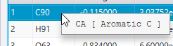
Right-click on each row in Non-Bonded Interactions field to view the details of the assignment.

NeuralMD¶

Set the Atomic Energy to without bias to activate the function that sets the bias terms of the last layer (which correspond to the internal energy of atoms) to 0. This adjustment levels the energy of the atoms.

The force field file designated in the Potential File setting can be generated using Advance/NeuralMD, or you can download and utilize pretrained force field files from the Force-Field Database.

Hint

The calculation of neural network force field can be accelerated using a GPU.

(Linux only) To execute calculations locally, specify the number of GPU(s) to be used in the Number of GPU setting, found under main menu ‣ Properties ‣ Advance/NeuralMD . If multiple GPUs are utilized, MPI parallel processes are evenly distributed across the GPUs.
To execute calculations remotely, enable the GPU setting in the queue of the ssh server setting.

Note

The installation of a GPU driver is required prior to use. Since CUDA 11.4.4 is being　utilized, a driver version of 470.82.01 or later is necessary.
In case where the system contains 5 or more elements, it is mandatory to use a weighted symmetry function during the generation of the force field.

Open Catalyst 2020¶

Utilize the pretrained versatile force field based on a graph neural network, which is publicly available in the Open Catalyst Project.

Since this feature operates by invoking Python from LAMMPS, it is essential to prepare the Python environment in advance. Additionally, there are some limitations to this approach. Click on info to view the detailed description.

MPI parallel processing is not supported (calculations using OpenMP parallel processing / a GPU are available).
ARM ver. (Apple M1) is not supported.
Periodic boundary conditions are not applied along the Z axis.
As virial stress is not calculated, calculations involving NPT/NPH ensemble or cell optimization are not supported.

Setting up the Python environment

M3GNet¶

Utilize the pretrained, versatile force field based on a graph neural network, which is published as M3GNet (original version, MatGL version) + correction by Simple DFT-D3.

Since this feature operates by invoking Python from LAMMPS, it is essential to prepare the Python environment in advance. Note that MPI parallel processing is not supported (OpenMP parallel processing / GPU are supported). Click on info to view a detailed description.

Setting up the Python environment

In Model, pretrained models bundled with M3GNet will be displayed. Also, you can import a model from the top left menu mainmenuicon by selecting Import ‣ Import M3GNet model.

CHGNet¶

Use pretrained versatile force field based on graph neural network, published as CHGNet + correction by Simple DFT-D3.

Since this feature operates by invoking Python from LAMMPS, it is essential to prepare the Python environment in advance. Note that MPI parallel processing is not supported (OpenMP parallel processing / GPU are supported). Click on info to view a detailed description.

Setting up the Python environment

In the Model section, pretrained models bundled with CHGNet will be displayed. Additionally, you can import a model by selecting Import ‣ Import CHGNet model from the mainmenuicon located at the top left.

SevenNet¶

Utilize the pretrained versatile force field based on a graph neural network, which is publicly available as SevenNet.

It supports multi-GPU, and is designed to run with 1 MPI process per GPU.

The LAMMPS executable file with SevenNet support is not included in NanoLabo. Follow the repository instructions to set up the runtime environment on a remote server, and prepare the executable file with the name lammps_sevennet. If necessary, set the PATH environment variable in the Job Script settings screen.

In Model, pretrained models bundled with SevenNet will be displayed. Also, you can import a model from the top left menu mainmenuicon by selecting Import ‣ Import SevenNet model.

SevenNet-0_serial: Capable of outputting stress.
SevenNet-0_parallel: Capable of multi-GPU execution. Cannot accurately calculate pressure.

Scheme¶

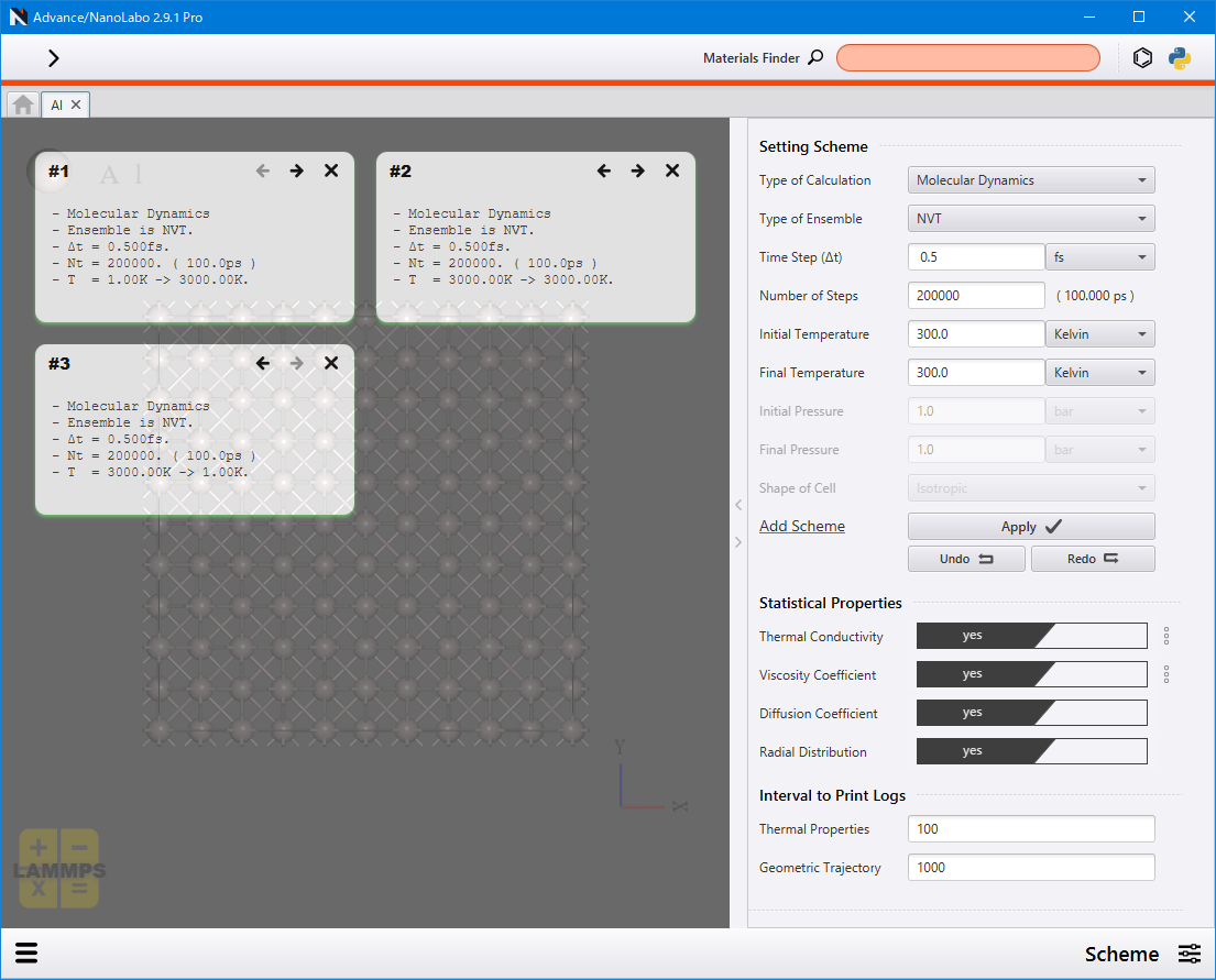
Configure the calculation scheme in the Scheme mode of the input file editor. Click on Scheme from the menu editormenuicon located at the lower right.

Set the parameters for the calculation scheme from the Setting Scheme on the right side of the screen.

Shape of Cell: Set the constraints on cell deformation for NPH and NPT ensembles.

Isotropic

Allow isotropic deformation

Anisotropic

Allow stretching along x, y, z axes

Triclinic

Allow arbitrary deformation

XY Isotropic

YZ Isotropic

XZ Isotropic

Allow stretching along the 2 axes at the same ratio

XY Anisotropic

YZ Anisotropic

XZ Anisotropic

Allow stretching along the 2 axes

XY Monoclinic

YZ Monoclinic

XZ Monoclinic

Allow arbitrary deformations in a plane containing the 2 axes

X Mobile

Y Mobile

Z Mobile

Allow stretching along 1 axis

Click Apply under Add Scheme to transfer the setting to the left side of the window as a tile. Repeat the process of configuring → Apply as many times as necessary to add multiple processes.

The number displayed on the upper left of each tile indicates the order in which the process will be executed. Use the back button lpback and the forward button lpfwd to change the order. To delete a process, use the delete button lpdel .

Shortcut keys are also available for some operations.

Operation
Remove the tile that was last added	`Ctrl` + `C` , `Backspace` , `Delete`
Undo	`Ctrl` + `Z`
Redo	`Ctrl` + `Shift` + `Z`

^* For macOS, replace Ctrl → command .

To edit the settings of an already added tile, double-click on it. This will deisplay the Set the scheme window, where you can modify the settings.

Additionally, by setting the options in Statistical Properties to yes, statistical quantities (thermal conductivity, viscosity coefficient, diffusion constant and radial distribution function (RDF)) will be calculated and displayed on the result screen. Parameters for thermal conductivity and viscosity coefficient can be configured via the dotsmenuicon menu.

Thermodynamic quantities and atomic structures are not output at every step, but rather at specified intervals. You can set these output intervals in the Interval to Print Logs by specifying the number of steps.

Option¶

Configure optional operations in the Option mode of the input file editor.

E-Field
Apply a static electric field.
Ext. Forces
Apply external forces.
Move Atoms
Move atoms at a constant speed, regardless of the forces acting on them.
Deform Cell
Deform the cell at a constant speed, with target atoms following the cell’s deformation.

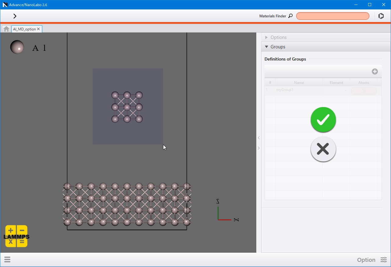
In each tab, select the target atom group using the Target Group , and then specify the relevant parameters.

These settings are specific to each Scheme , and are only applied to the selected Target Scheme .

Hint

To move atoms by setting initial velocities, you shuld not use this screen. Instead, go to Velocities section under Geometry .

Initially, you can only select “all” (all atoms) as the Target Group . To define additional atom groups, navigate to Groups . Click add to add a new row, and then choose Element to select multiple atoms at once, or click Atoms to select atoms individually. To delete atom group, click Delete from the right-click menu of the row.

Note

Due to LAMMPS specifications, the maximum number of atoms groups is limited to 32 (you can add up to 31, excluding “all”).

User’s¶

Configure additional user commands / variables for output and plotting.

User’s Additional Settings into Input-file
Add any LAMMPS commands into the text box to insert them to the input file.
User’s Variables to Output and Plot
When you add a variable, a corresponding button will be added to the result view, allowing it to be desplayed as a time-series plot. Additionally, a corresponding column for this variable will be added to the CSV file.

You can use pre-defined variables (as referenced in the LAMMPS manual) or variables added via LAMMPS command.

For instance, in a calculation where bonds / angles are defined (OPLS-AA force field), the setting below allows for plotting the average bond length / angle, while also outputting the histgram to a file at each timestep.

User’s Additional Settings into Input-file

compute 1 all bond/local dist
compute 2 all angle/local theta
compute 3 all reduce ave c_1 c_2
fix 1 all ave/histo 10 10 100 0.8 1.1 20 c_1 mode vector file dist.histo
fix 2 all ave/histo 10 10 100 80 120 20 c_2 mode vector file theta.histo

User’s Variables to Output and Plot

c_3[*]

Please refer to LAMMPS manual for guidance on the usage of LAMMPS commands.

Isotropic	Allow isotropic deformation
Anisotropic	Allow stretching along x, y, z axes
Triclinic	Allow arbitrary deformation
XY Isotropic YZ Isotropic XZ Isotropic	Allow stretching along the 2 axes at the same ratio
XY Anisotropic YZ Anisotropic XZ Anisotropic	Allow stretching along the 2 axes
XY Monoclinic YZ Monoclinic XZ Monoclinic	Allow arbitrary deformations in a plane containing the 2 axes
X Mobile Y Mobile Z Mobile	Allow stretching along 1 axis