Result

Once the calculation is initiated, you can review the results in the project tab, where the results ready for visualization are listed as tiles. (If the result view is not displayed, click the Result from the menu on the lower left to open it.)

Click on the item you wish to view to open the result view. To return to the list, click back button on the lower left.

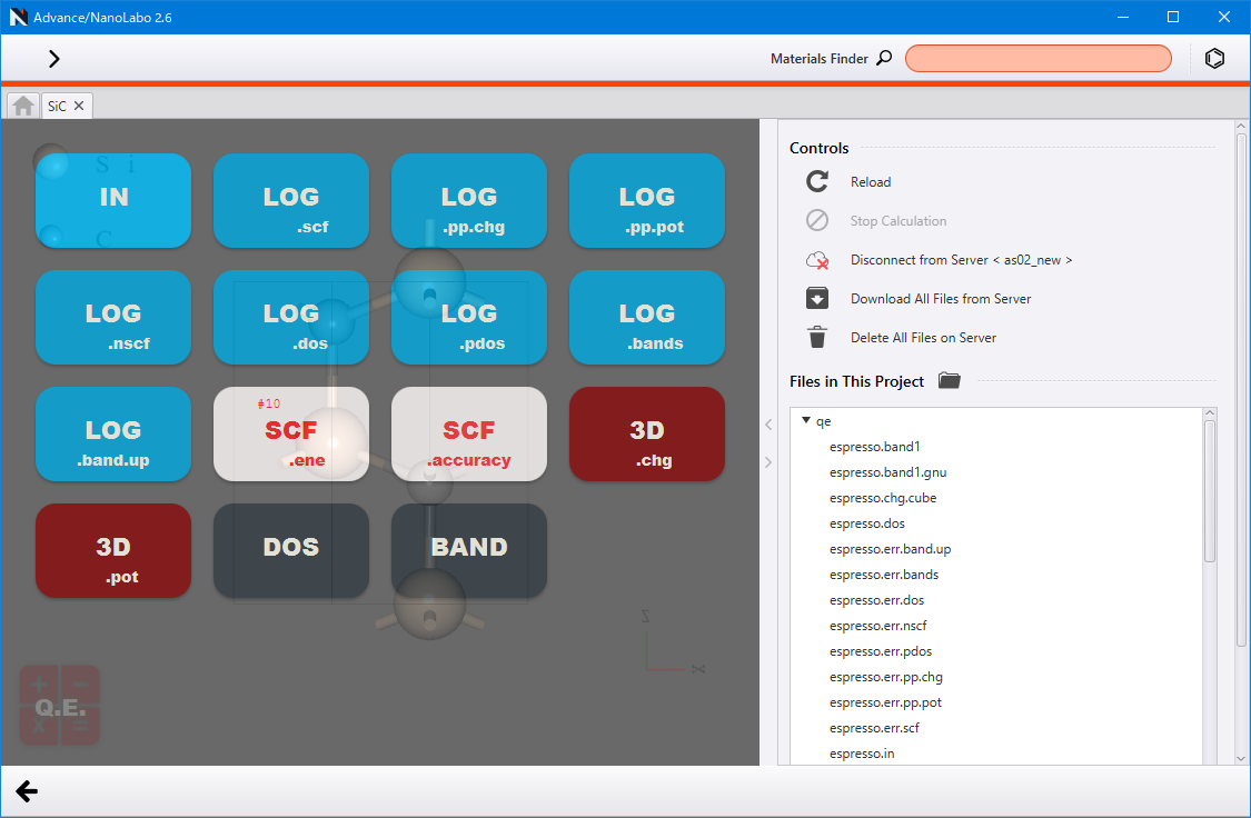
If the calculation is running on the remote server, the results are continuously fetched while the result view is open.

Click the Disconnect from Server icon on the right side panel to suspend access. Automatic downloads are performed only for the files required for visualization. To manually download all files in the project, click Download All Files from Server icon. If file capacity is a concern on the server, you can use Delete All Files on Serveroption to remove them.

If always offline mode is enabled in the SSH server setting, access will be suspended when you open the result view. However, even in this status, if a Download Time is set, the files will be fetched at that interval. While fetching is in progress, the icons will change to .

Click the icon on the right of Files in This Project to open the project folder with an external filer (a local folder will open even if executed remotely).

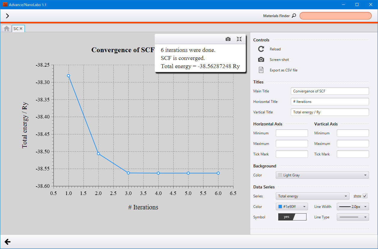
2D plot

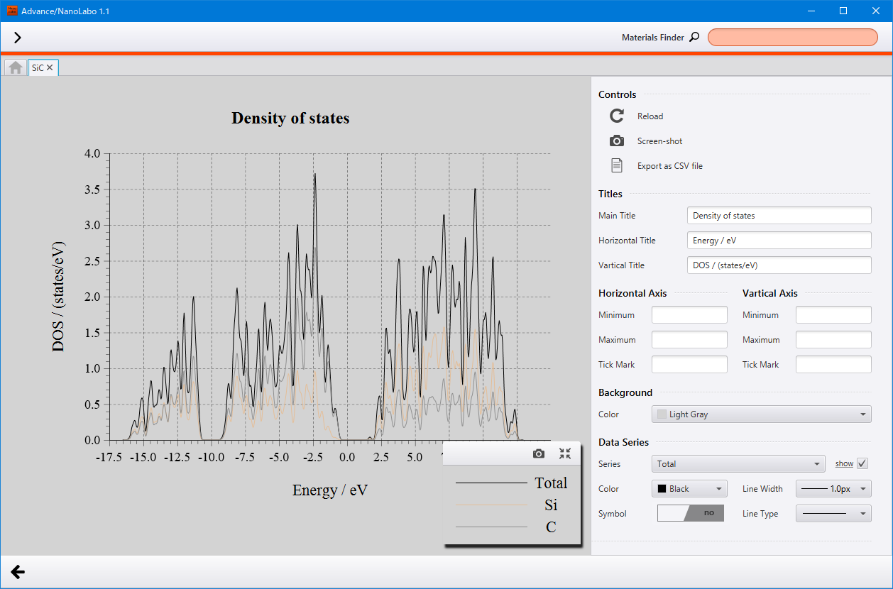
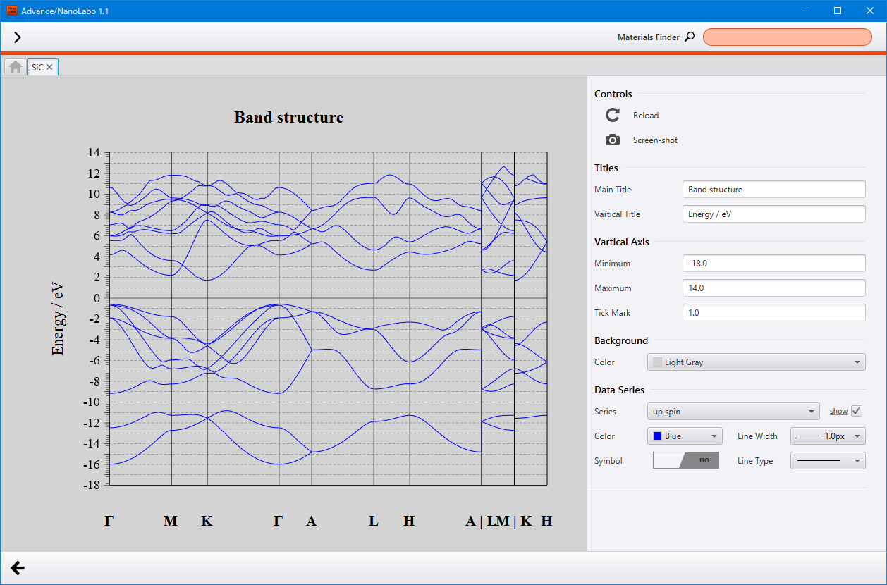
Time series data, density of states, or band structure are displayed in a 2D plot. Adjust the plot appearance using the right side panel. In the Data Seriessection, you can select which data series to display and tweak their appearance.

You can customize the density of states plot using the PDOS Calculator.

• PDOS Calculator

If the calculation is running, click Reload to read the output file and update the display.

Click Screen-shot to save the plot as an image file. Click Export as CSV file to save the displayed data as a CSV file.

Hint

In the time series plot of LAMMPS, some data points may not be displayed to enhance performance when there are too many data points. To adjust this setting, open Properties ‣ LAMMPS from the in the upper left and toggle Data to Plot Graphs .

3D display

Click the 3D buttons to visualize the spacial distribution of charge density / potential / spin polarization (if spin is enabled) obtained from SCF calculation in 3D.

They can by visualized using Isosurface or Cloud. The list of rendered objects is displayed in the right side panel. The objects can be shown / hidden using the , and you can adjust the display setting using . You can add or remove the object using the or .

Click the button under Referential Data and select the data (project / cube file) previously calculated to display the difference. The mesh division number must be the same. If you set two sets of data, the values from both are subtracted (current - #1 - #2) and displayed.

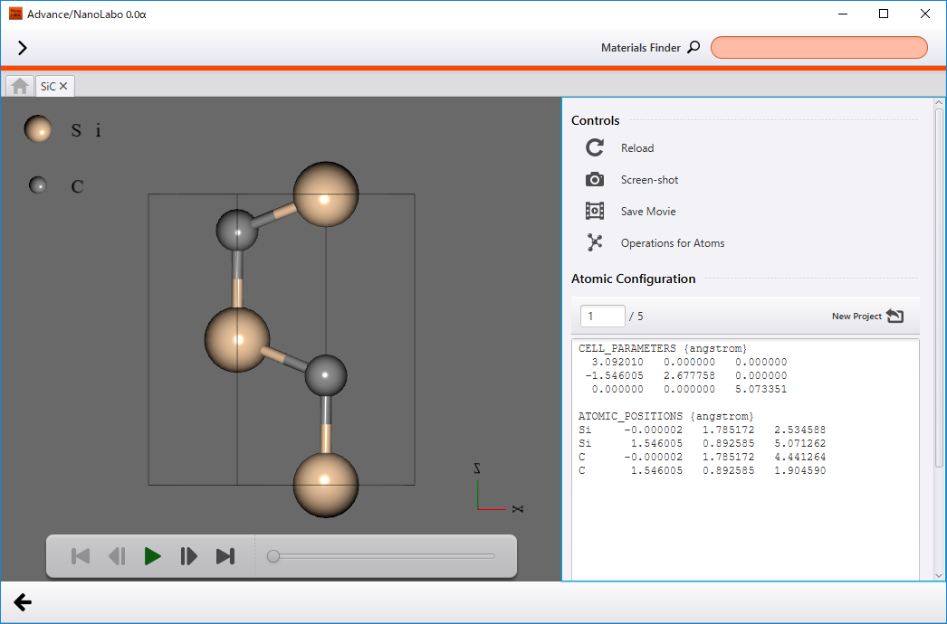
Movie

Click .movie to display the change in atomic structure as an animation. If the calculation is running, click Reload to read the output file and add updated frames.

You can change the viewpoint in the same way as in the atomic structure viewer. You can also adjust the viewpoint even during playback.

Click Screen-shot to save the current frame as an image file. Click Save Movie to save all the frames as a movie file.

Click New Project to create a new project using the current atomic structure and start the analysis.

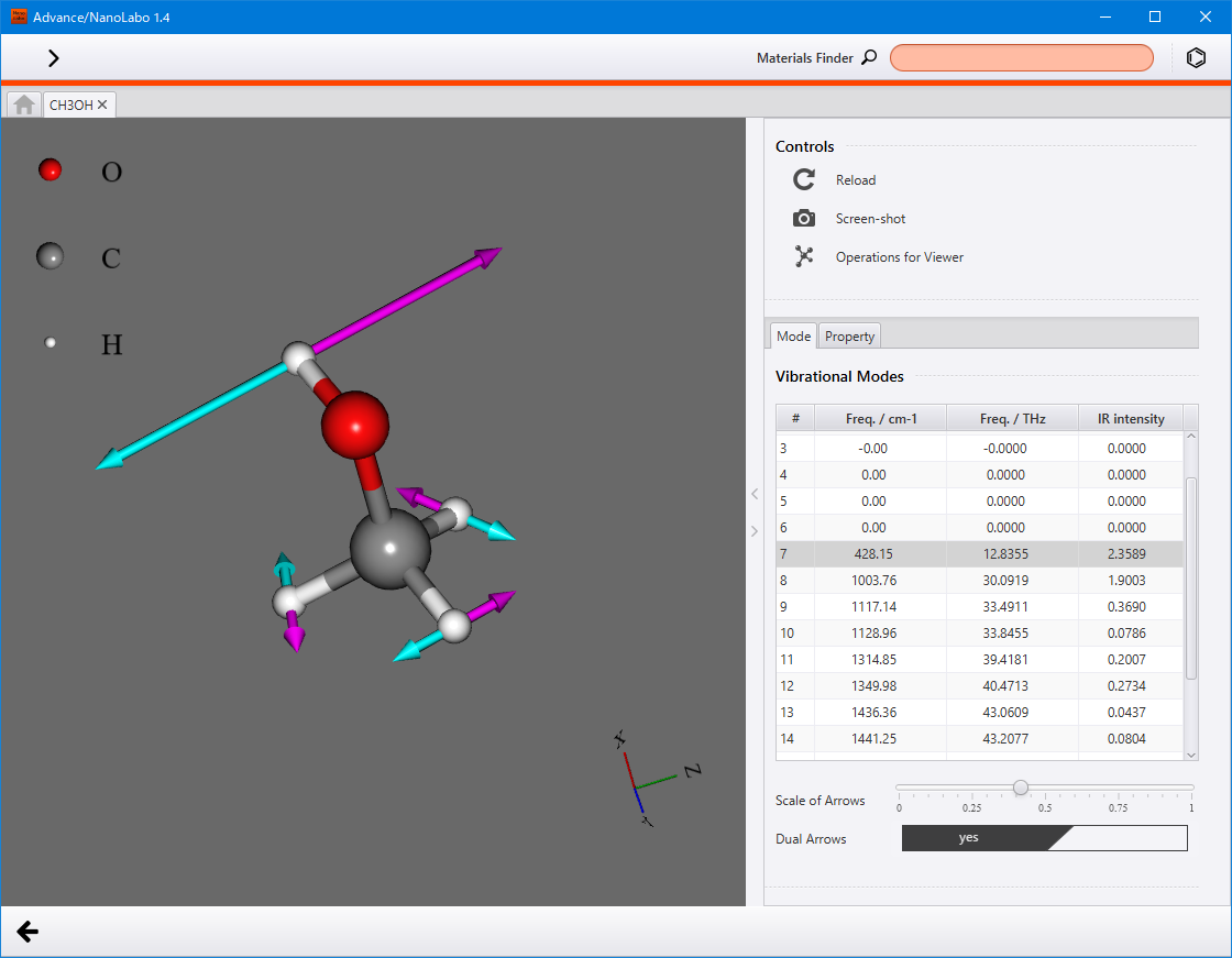
Phonon modes

Click Phonon.mode to visualize each vibrational mode with arrows.

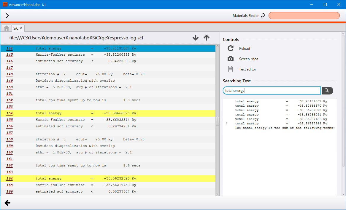
Text

Click IN (input file), LOG (log file), ERR (error log file) to display the contents of the file. You can utilize in-file search, highlighting and extracting features.

Click Text editor to open the file with an external text editor.

Update atomic configuration

After performing a calculation involving changes in atomic configuration, click Update to refresh the project’s atomic configuration to the modified one.