Input File Editor (Quantum ESPRESSO specific settings)¶

Pseudopotential¶

For pseudopotential settings, select Geometry from the menu editormenuicon in the lower right, then find Element’s Properties in Elements. Click the button in the Pseudopotential column corresponding to the element you wish to configure. Below the table, you will find the suggested cutoff energy.

To add a pseudopotential file, go to the top-left menu mainmenuicon and select Import ‣ Import Pseudopotential.

After changing the pseudopotentials, navigate to the SCF setting, and click the default value button default in the Cutoff field to input the updated suggested value for the cutoff energy.

Path of the band calculation¶

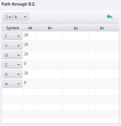
When you select Band or Ph. Dispersion from the menu editormenuicon in the lower right, you will find Path through B.Z. among the available settings. The method for configuring this setting is described.

In the Symbolfield , specify the points you want to go through. If you need to specify a point that is not in list box, leave the Symbol field empty and enter the coordinates in kx, ky, kz (or qx, qy, qz ).

You can add, delete or reorder the points using the right-click menu of each row. When you add a point, a new row is inserted immediately following the clicked row.

In the nk (or nq ) field, specify the number of points to be calculated between the points specified in that row and the next row. For example, in the first row in the image, nk is 20, indicating that calculations will be performed at 20 points between the Γ point specified in that row and Y point specified in the next row.

If nk is set to 0, no calculations are performed between the points specified in that row and the next row. On the band diagram, the points from that row and the next row will be displayed as merged.

ESM method¶

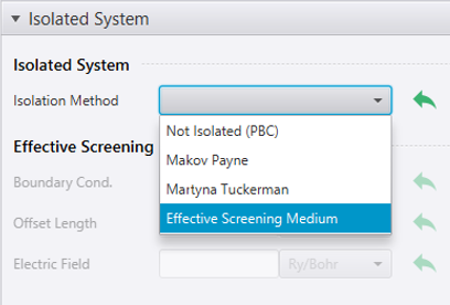
Select SCF from the menu editormenuicon in the lower right. Then, in the Isolated System section, choose Effective Screening Medium from the Isolation Method menu.

The selection of the ESM method may cause the atomic positions to be adjusted in the direction normal to the surface for computational convenience.

NEB method¶

When you select NEB from the menu editormenuicon located at the lower right, you will find Images among the available setting. You can configure initial images for the NEB calculation. The method for configuring this setting is described.

Initially, only the first image is set, and it is identical to the current project. To add additional images, click add and select a project to set as the last image. Intermediate images will be automatically added in between.

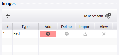
The buttons on each row allow the following operations:

Click to insert an image. A new image is inserted after the selected one.
Click to remove an image.
Click and select a project to replace an image with another.
Click to highlight an image.

Additionally, you can click to_be_smooth to smoothen a series of images.

Hint

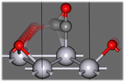
For correct NEB calculation, corresponding atoms of each image must be listed in the same order in the input file. When adding images, atom ordering is automatically adjusted based on atomic bonds. This algorithm can be adjusted via the settingicon button.

Bond Watching: Controls whether to perform reordering of atoms when adding an image. Set to no to use the original input file’s atom sequence.
Bond Scale: Coefficient used to determine the presence of bonds from atomic distances.

XAFS¶

When you select XAFS from the menu editormenuicon located at the lower right, you will find XAFS-specific settings. In this section, XAFS-specific configurations are described.

The use of a Super Cell is essential to maintain a sufficient distance between neighboring excited atoms. In case where the cell is small, an excited atom may be influenced by an excited atom in a neighboring cell due to periodic boundary condition. To prevent this, the cell is automatically converted into an appropriate super cell based on the cell size.

To select the atom to be excited, use Target Atom. Click Select Atom and choose an atom by double-click. Once you’ve finished selecting the atom, it will be displayed on the button when you click End Selecting Atom.

Next, click the Core-hole P.P. button to select the pseudopotential for the excited atom. It is important to choose a pseudopotential with a hole in the core orbital (Core-hole pseudopotential). Please note that Core-hole pseudopotentials are not included in the NanoLabo Tool. If needed, you can download them using Download button. The files are typically named as “star + orbital name”(star1s, for example) to indicate the location of the hole (= from which orbital it is excited).

Additionally, for XAFS calculations that rely on core orbital wave function information, it is necessary to use the GIPAW pseudopotential, which contains that information. To do this, go to the menu editormenuicon in the lower right, then navigate to Geometry ‣ Elements and set GIPAW pseudopotential for the element corresponding to the excited atom. These pseudopotential files typically include “gipaw” in their file names.

CPMD¶

Select MD from the menu editormenuicon located at the lower right, then open the CPMD tab and set Car-Parrinello to yes. This will enable you to perform Car-Parrinello molecular dynamics calculation.

The SCF calculation of the electronic state is conducted initially, followed by the time evolution of both the electronic state and the atomic structure. You can select the method for the initial SCF calculation using Initial SCF. The other parameters of electronic state calculations are configured by referring the settings in the SCF screen, with possible modifications to account for the limitations of CPMD.

Additionally, please note the following limitations regarding pseudopotential:

When using ultrasoft pseudopotential, the box grid must be configured.
PAW pseudopotential cannot be used.

NMR spectrum¶

When you select GIPAW from the menu editormenuicon located at the lower right, you will find NMR spectrum settings.

Set Macroscopic Shape to yes to apply the correction related to the macroscopic shape of the sample. Specify the correction along each axis by Shape Tensor.

You can also specify the shielding tensor of the reference compound $\sigma_\mathrm{ref}$ in the result plotting screen.

Phonon Dispersion¶

When you select Ph. Dispersion from the menu editormenuicon located at the lower right, you will find phonon dispersion settings.

Set Calc. DOS in the DOS tab ( Calc. Band in BAND tab) to perform calculation of phonon density of states (phonon bands).

You can account for LO-TO splitting by setting Non-Analytic Term to yes. To enable the correction, the Born effective charge must be obtained in advance by calculating Phonon at the Γ point (qx, qy, qz) = (0, 0, 0) and the Dielectric Constant , Effective Charge set to yes. If the Born effective charge is not calculated, the calculation will Proceed without correction, even if Non-Analytic Term is set to yes.